Introduction

FLUX.1 ¹ is a Rectified-Flow transformer trained in the latent space of an image encoder, introduced by Black Forest Labs in August 2024.

The FLUX.1 models demonstrate State-of-the-art (SoTA) performance for text-to-image tasks, in both terms of output quality and image-text alignment, as demonstrated in Figures 1 and 2 using the ELO-score metric, which ranks image generation models based on human preferences in head-to-head comparisons.

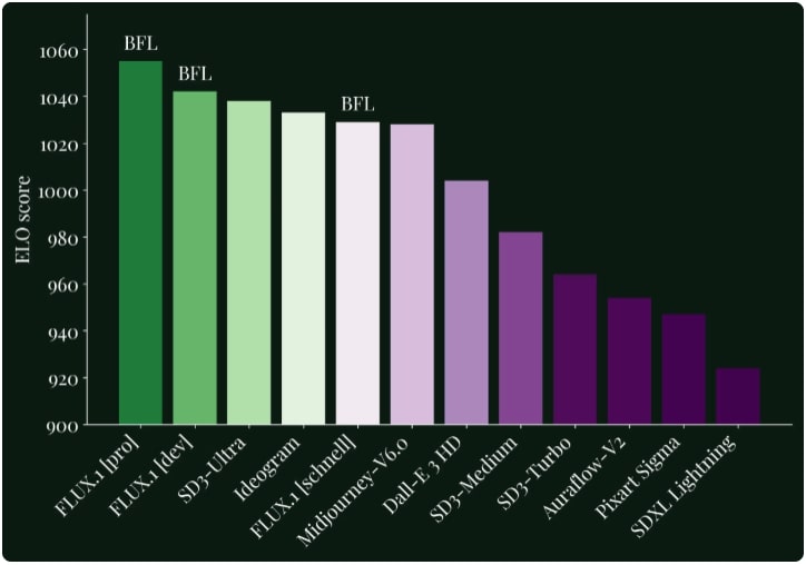
Figure 1. FLUX.1 defines a new state-of-the-art in image detail, prompt adherence, style diversity and scene complexity for text-to-image synthesis. Evaluation from ²

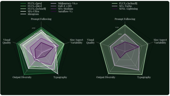
Figure 2 ELO scores for different aspects: Prompt Following, Size/Aspect Variability, Typography, Output Diversity, Visual Quality. Evaluation from ²

While the model adheres to the Rectified Flow training paradigm (according to the developers statement), the exact details regarding the training setup —including the dataset, scheduling strategy, and hyperparameters— have not been publicly disclosed. However, the model’s architecture and inference scheme can be reverse-engineered from the publicly available inference code.

In this section, we outline the model’s architecture to demystify its behavior at inference time. A top-view of the architecture is illustrated in Figure 3, where text embeddings and latent image embeddings are iteratively processed via a series of attention blocks. In the following section we deep-dive into the different components of the model.

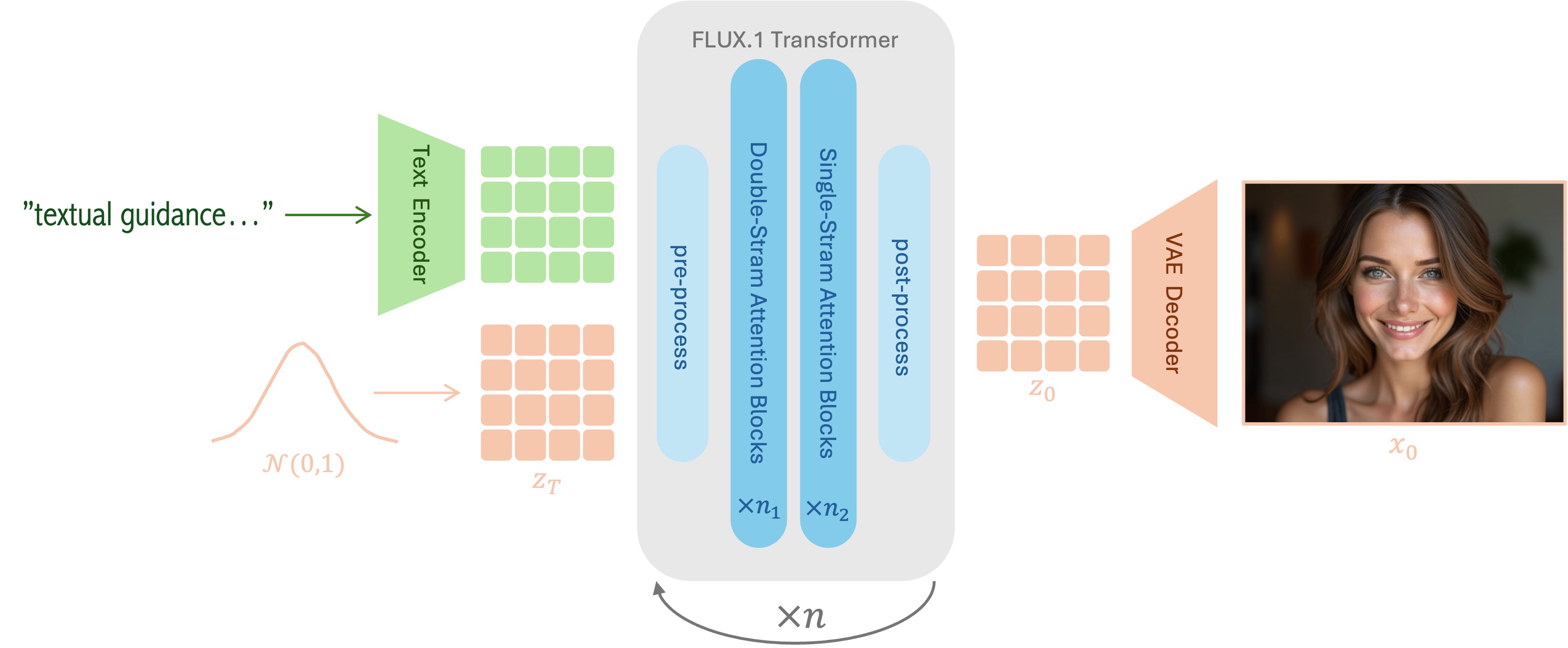
Figure 3. High-level overview of the FLUX.1 architecture. Text embeddings and latent image embeddings are iteratively processed through a series of attention blocks to generate a text-conditioned image.

In the following section we deep-dive into the different components of the model. We begin with a high-level overview of FLUX’s sampling pipeline in FLUX.1 Sampling Pipeline, highlighting the key stages and the pre-trained components involved, followed by a deep-dive into the transformer’s architecture in Transformer, where a detailed explanation is provided to the different stages and concepts used to construct it.

---

FLUX.1 Sampling Pipeline

In this section, we describe the sampling pipeline of FLUX.1. For simplicity, we refer to the text-to-image sampling process as being conditioned on a single prompt per sample.

Similar to LDM ³, FLUX operates in a latent space, where the final latent output is decoded to reconstruct the RGB image in pixel space. Following LDM’s approach, the developers trained a convolutional autoencoder from scratch using an adversarial objective, but scaled up the latent representation from 4 channels (in LDM) to 16 channels.

The sampling pipeline consists of three phases: \((1)\) Initiation and Pre-processing \((2)\) Iterative Refinement, and \((3)\) Post-processing. An overview of these steps is illustrated in Figure 4, where the notations follows the ones used in the official implementation of FLUX.1 pipeline in the diffusers ⁴ library.

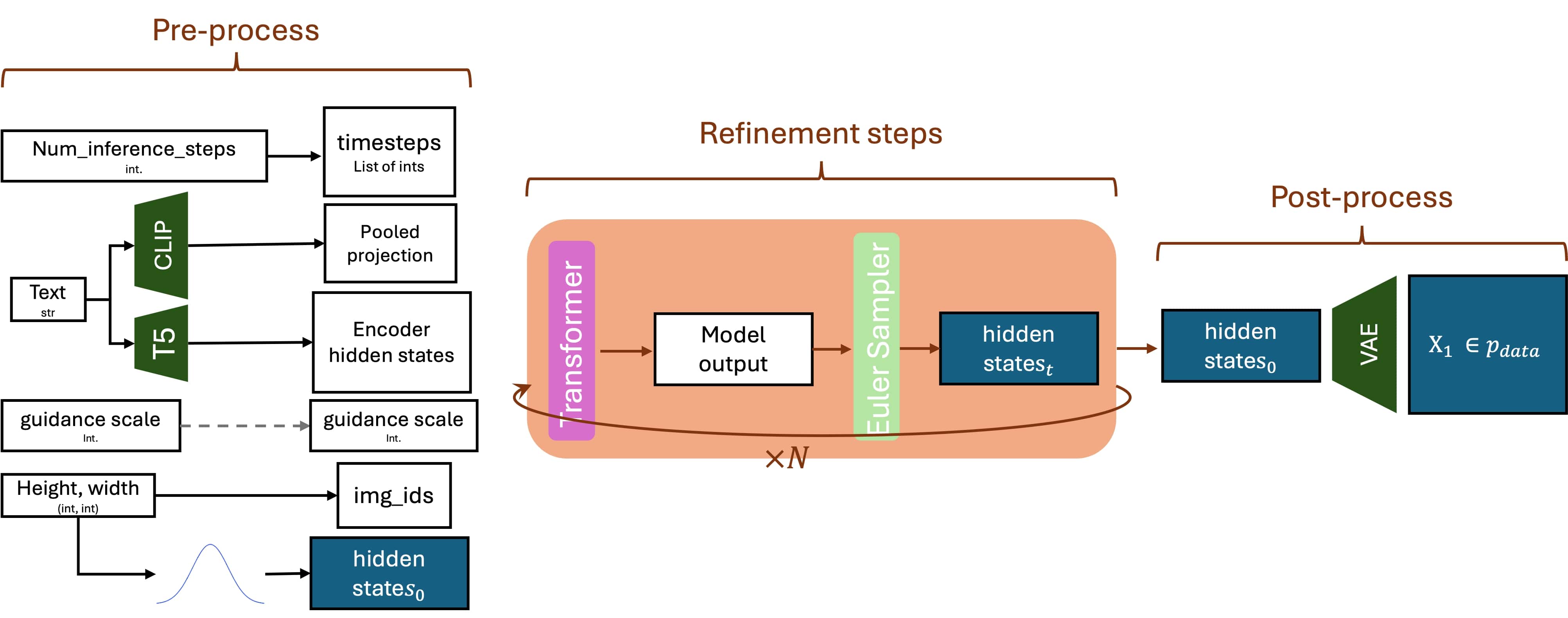
Figure 4 Flux pipeline: high-level overview. Just like in Difussion Models, after pre-processing the noisy latent $z_t$ (denoted hidden_state$_t$) is being iteratively refined in the latent space, the final refined \(z_0\) (\(=\)hidden_states\(_0\)) is decoded into an RGB image using a pre-trained VAE decoder.

In the section below, we primarily focus on the Initiation and Pre-processing phase of the pipeline. A brief overview of the Iterative Refinement and Post-processing phases is provided at the end of this section. The Iterative Refinement phase, in which the FLUX transformer operates, is discussed in detail in Section Transformer.

Initiation and Pre-processing

In this phase, the model processes the user-provided inputs to prepare them for the main transformer’s refinement stage. A key component of this stage is the text encoder, which processes the textual guidance supplied by the user. FLUX.1 utilizes two pre-trained text encoders:

CLIP Text Encoder. CLIP (Contrastive Language–Image Pretraining) ⁵ is a foundation model developed by OpenAI, designed to bridge vision and language understanding. CLIP’s text-encoder transforms natural language prompts into class level or dense, high-dimensional embeddings that can be directly compared with image embeddings in a shared latent space. Trained on hundreds of millions of image–text pairs, the CLIP text encoder captures rich semantic information, enabling models to align textual descriptions with corresponding visual content effectively, making it widely used in text-to-image generation tasks.

T5 Text Encoder. T5 (Text-To-Text Transfer Transformer) ⁶ is a versatile language model developed by Google that frames all NLP tasks (e.g., translation, summarization, and question answering) as text-to-text problems. Its text encoder converts input text into contextualized embeddings using a Transformer-based architecture trained over massive language corpora. Unlike CLIP’s text encoder, which is trained jointly with an image encoder to produce embeddings aligned with visual features for contrastive learning, T5 is trained purely on textual data and optimized for language understanding and generation. This makes T5 well-suited for providing rich, token-level semantic representations even for long and complex textual prompmts.

Below, we outline all the required inputs and describe how the model processes them in preparation for the refinement stage. The pipeline’s inputs are:

• text: textual prompt guides the image generation process to enforce specified features or qualities.
• guidance_scale: controls the strength of conditioning.
• num_inference_steps: how many iterative sampling steps should be performed.
• resolution: Specifies the spatial resolution (height and width) of the generated image.

Once initiated with those inputs, they are being preprocessed as follows (notations are borrowed from the official implementation by diffusers ⁴):

• text: The textual prompt is being encoded using two pre-trained text encoders:
  • T5: provides dense (per token) embeddings, denoted encoder hidden states
  • CLIP: provides pooled embeddings (one embedding for the whole prompt, like CLS embedding), denoted pooled projection

• num_inference_steps: Specifies the total number of sampling steps used during inference. It determines a subset of timesteps from the full diffusion range \(t \in [0:T]\), where typically \(T=1000\). Iterating over these selected timesteps defines the sampling trajectory.

• resolution: The desired resolution determines the spatial dimensions of the initial (latent) noise sample \(z_0 \sim \mathcal{N}(0,1)\). It is also used to define the img_ids — a set of per-token indicators, pointing at the token’s spatial location on a 2D grid. Given a target resolution \((H,W)\) in pixel space, the corresponding latent dimensions \((h,w)\) are computed as \(h = \lfloor H / \text{VAE_scale} \rfloor\) and \(w = \lfloor W / \text{VAE_scale} \rfloor\) where \(\text{VAE_scale}=8\).
  The image-token grid is further downsampled to dimensions \((h//2, w//2)\), and each token is assigned a unique identifier of the form \((t, \hat{h}, \hat{w})\), where \(\hat{h} \in [0:h-1]\) and \(\hat{w} \in [0:w-1]\), indicating the token’s location on a 2D spatial grid.
  text_ids are initiated using the same structure of img_ids, but with \(t = h = w = 0\) for all tokens. Formally, \(\text{text_ids} = n \cdot (0,0,0)\) where \(n\) is the maximal number of tokens in T5 (512).

Iterative Refinement and Post-processing

Let \(\Phi = [\text{encoder_hidden_states}, \text{pooled_projection}, \text{guidance}, \text{img_ids}, \text{text_ids}]\) be a set the pre-processed pipeline’s inputs. Same as in Diffusion Models, \([z_t, t, \Phi]\) are iteratively fed into the transformer during inference sampling, such that:

\[\forall t \in \text{timesteps}: \quad z_{t+\Delta t} = \text{Samp}\bigl(v_\theta(z_t, t, \Phi)\bigr)\]

Where \(v_\theta\) is the trainable network that estimates the velocity vector (see Rectified Flow) and \(\text{Samp}(\cdot)\) refers to the Flow-Matching Euler Discrete sampler [^lipman2022flow]. Pay attention to the notation that differs from the one used in Diffusion Models. Here timesteps range between \(0\) and \(1\), with \(z_1\) the clear image and \(z_0\) the pure Gaussian noise. In Section Transformer we explore the architecture of \(v_\theta\).

After the iterative refinement, the final clean latent \(z_1\) is decoded via pre-trained VAE model to get the final image \(x_1\).

---

Transformer

The core component of FLUX.1’s synthesis pipeline is the velocity predictor \(v_\theta\), which is optimized to estimate the velocity vector along the sampling trajectory (see Section Rectified Flows). Similar to SD3 ⁷, FLUX.1 replaces the conventional U-Net architecture with a fully transformer-based design.

A high-level overview of the transformer’s operations at each sampling step is provided in Figure 5 using the notation defined in the official implementation by diffusers ⁴.

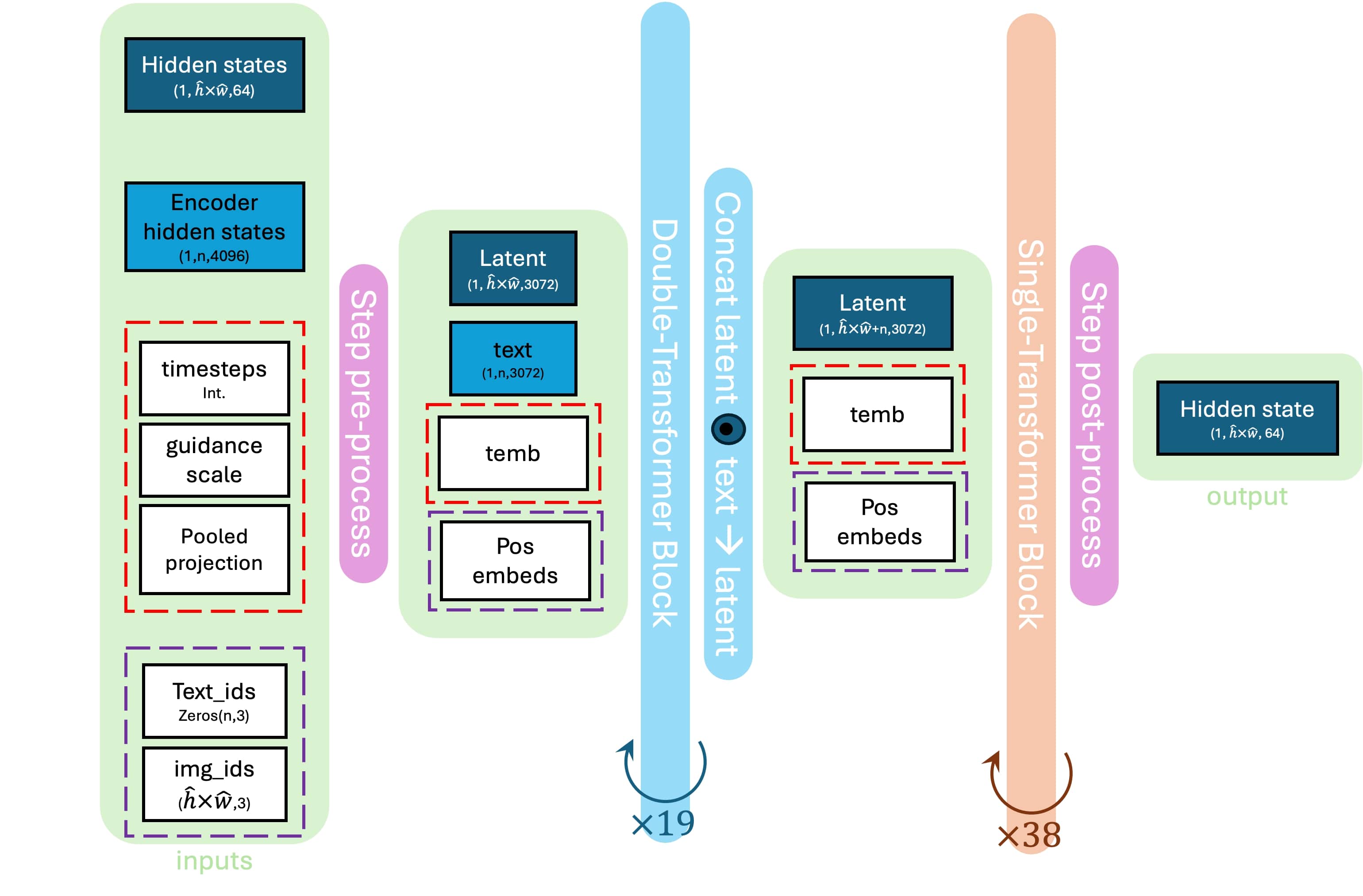Figure 5 Flux Transformer: high-level overview.

On every iteration, the inputs are preprocessed before they ate fed into a sequence of transformer blocks.

There are two types of transformer blocks: \((1)\) Double-Stream (see Section Double Transformer Block), and \((2)\) *Single-Stream (see Section Single Transformer Block.

Both blocks employ Multi-Modal Attention: a joint self-attention mechanism to process concatenated text and image tokens in a unified attention operation, enabling bidirectional interactions that capture both self-information and cross-modal information between text and image modalities. Below we provide a step-by-step guide to the per-iteration pre-process, and the Double-Stream and Single-Stream attention blocks.

Per-Iteration Pre-process

Along the sampling trajectory, the transformer is called multiple times, once at each sampling iteration. In every call, it is provided with an updated set of parameters:

• The guiding parameter timestep is iterated from the pre-calculated list of values between 1 to 0.
• hidden_state (mostly referred to as \(z_t\)) is the latent representation which is iteratively refined from Gaussian noise into a clear image. It is updated along the sampling trajectory.

These parameters join the ``constant” inputs (which remain constant across different iterations) pre-calcualted in the pipeline’s pre-process stage (See section Initiation and Pre-processing). The transformer pre-processes it’s inputs internally as described in Figure 6:

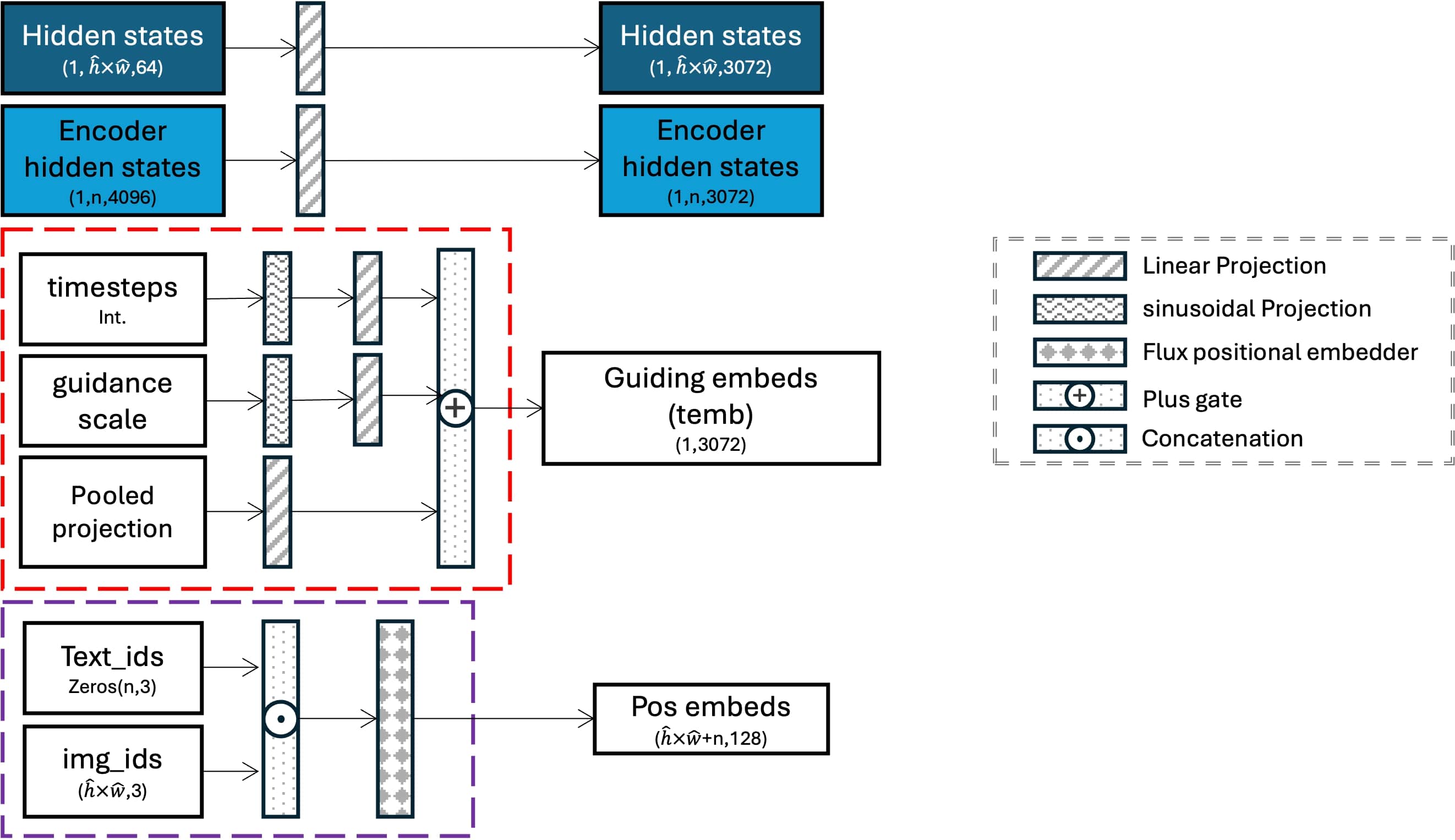Figure 6 Flux Transformer: per-step inputs preprocess

Formally, the following steps are taken:

• use of per-domain linear layers to bring the latent embeddings and dense-prompt-embeddings (T5) into a shared dimensionality of 3072 features per token.
• construction of guiding embeds. Unlike Diffusion Models, that encode only the ``temporal” information (i.e, timestep) in this phase, FLUX.1 uses both the timestep and the pooled prompt embeds (from CLIP) as guiding embeddings, yet keeps the traditional notation temb. It uses sinusoidal projection (As in ⁸) to embed the integer values of the timestep and guidance, than applies dedicated linear projection layers to each component to bring them to the shared dimensionality of 3072 features. Finally, the 3 projected embeddings are summed to create the final temb (marked in a red block in Figure 6).
• The img_ids and text_ids (see Section FLUX.1 Sampling Pipeline)are concatenated, than used to extract per-token positional embeds. To extract positional embeddings from 3D token indices (t,h,w), each axis is first converted to a continuous embedding using axis-specific sinusoidal frequencies scaled by a constant \(\theta\). he cosine and sine of the resulting frequency-position products are computed and interleaved to form real-valued vectors. These are then concatenated across all axes to produce the final positional embedding as a pair of tensors (cosine and sine), ready to be used in rotary positional encoding (the process os composed in the purple block in Figure 6). Note that this process is not influenced neither by timestep nor hidden_states, hence the pos_embeds are constant across different sampling steps.

The pos_embeds and temb parameters are used to support the attention mechanism along the step, while hidden_states and encoder_hidden_states are processed and refined along the step.

---

Double-Stream Transformer Block

After preprocess, a series of 19 Double-Stream Transformer blocks are applied. Those blocks employ separate weights for image and text tokens. Multi-modality is achieved by applying the attention operation over the concatenation of the tokens, ass iluustrated in Figure 7b.

Those blocks employ seperate weights for image and text tokens (see Figure 7a). Multi-modality is achieved by applying the attention operation over the concatenation of the tokens (see Figure 7b).

Figure 7a. Double-Stream Attention Block: latent and prompt embeddings are processed separately, in a standard multi-modal attention scheme.

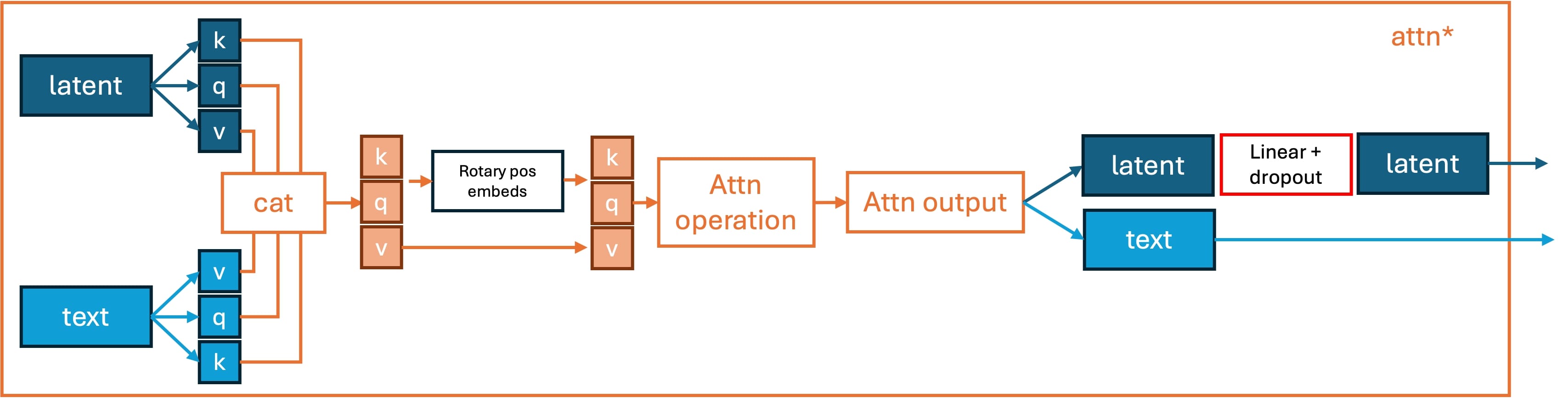Figure 7b. The attention operation is applied over the concatenation of the tokens.

Each stream (latent and prompt) uses Adaptive Layer Normalization (AdaLN) ⁹ layers for normalization and modulation (see Figure 7a and in details in Figure 8).

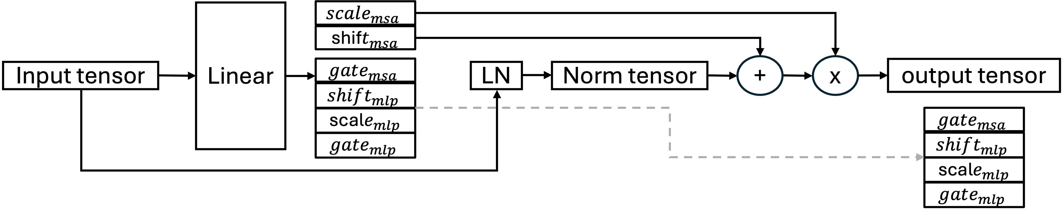
Figure 8 AdaLN layer, where MSA (Multi-head Self Attention) and MLP (Multi-Layer Processor) modulation parameters are computed based on the input tensor. In Single-Stream block (see Section Single-Srteam Transformer Block), MLP modulation is not computed.

AdaLN is a conditioning mechanism used in Transformer-based models ^{10 11} to modulate intermediate activations based on external input, such as text or image embeddings, based on the Adaptive Instance Normalization (AdaIN) mechanism proposed in to modulate intermediate activations based on external input, such as text or image embeddings, based on the Adaptive Instance Normalization (AdaIN)¹². Unlike standard Layer Normalization, which applies fixed scaling and shifting parameters, AdaLN dynamically generates these parameters as functions of a conditioning vector (see Figure 8). This allows the model to adapt its behavior at each layer according to the input prompt or guidance signal.

The normalized tensors are used to extract the \(K\), \(Q\), and \(V\) matrices for each domain, which are then concatenated for mixed attention. The concatenated \(K\) and \(Q\) matrices are rotated using precomputed Rotary Positional Embeddings. Rotary Positional Embeddings (RoPE) ¹³ are a method for injecting positional information into Transformer models by rotating the query and key vectors in multi-head self-attention according to their token positions. Unlike traditional sinusoidal or learned positional embeddings that are added to input tokens, RoPE applies a rotation in the complex plane that preserves relative positional relationships across sequences. This approach allows the model to generalize better to unseen sequence lengths and supports extrapolation beyond training data. RoPE has become popular in recent vision-language models, where understanding spatial relationships between tokens, especially when re-purposing textual positions for image patches, is crucial.

The rotated \(K\) and \(Q\) matrices are passed through the mixed attention operation. The outputs are separated back into their respective streams and alpha-blended with the residual input using the \(gate_{\text{msa}}\) parameter, extracted by the AdaLN layer. The results are further normalized via a LayerNorm (\(LN\)) layer and modulated using the \(scale_{\text{mlp}}\) and \(shift_{\text{mlp}}\) parameters, also extracted by the AdaLN layer, before being passed to the feedforward layer. Finally, the output is alpha-blended with the unnormalized input using the \(gate_{\text{mlp}}\) parameter from the AdaLN layer. The entire process is illustrated in Figure 7a.

---

Single-Stream Transformer Block

After the series of Double-Stream blocks is applied, the processed latent and prompt embeddings are concatenated and fed through a series of Single-Stream blocks.

While the Double-Stream blocks apply different weights for prompt and latent embeddings, the Single-Stream blocks use a single set of weights to process a concatenated tensor or latent and text embeddings (see Figure 9a). In addition, the Single-Stream blocks replace the standard sequential attention block (where an MLP, like Feed-Forward is applied after the attention step), with a parallel mechanism where the attention block and an MLP are computed simultaneously from the same input.

Figure 9a. Single-Attention Block: latent and prompt embeddings are processed together, in a simultaneous attention scheme.

Figure 9b. The \(K\), \(Q\) and \(V\) metrices are computed directly from the concatenated representation.

This “parallal attention” mechanism should not be confused with the multi-modal attention mechanism, which is used in both Double-Stream and Single-Stream blocks, where self-attention and cross-attention are computed jointly in parallel (see Figures 7b and 9b).

A comparison between the Double-Stream and Single-Stream blocks is summarized in Table 1:

| Property | Double-Stream Block | Single-Stream Block | |——————–|————————————————————————————|——————————————————————————-| | Weight Sharing | Uses separate weights for text and latent tokens in both attention and feedforward layers. | Uses shared weights for both text and latent tokens across attention and feedforward layers. | | Computation Style | Attention and feedforward (MLP) layers are applied sequentially, where the attention’s output defines the feedforward’s input. | Attention and feedforward layers are computed in parallel using the same input for both. |

Table 1: Comparison between Double-Stream and Single-Stream blocks in FLUX.1

Specifically, the Double-Stream and Single-Stream blocks differ in two main attributes: weight sharing between text and latent tokens (shared vs. not shared), and computation style (sequential vs. parallel). While the exact motivation behind the FLUX.1 developers choice of this specific architecture is not documented, the following is a brief comparison of these attributes, highlighting the possible pros and cons of each, potentially shedding light on the reasoning behind including both block types in FLUX.1’s architecture.

Weight Sharing (Shared vs. Not Shared)

Weight sharing refers to whether the same attention and feedforward parameters are used for both text and latent tokens. In the Single-Stream block, shared weights enable more efficient parameter usage and promote tighter integration between modalities, which may help the model generalize better across domains. However, this comes at the cost of reduced flexibility, as both token types must be processed identically despite potentially having very different characteristics. In contrast, the Double-Stream block avoids weight sharing, allowing the model to specialize its representations for text and latent tokens independently. This specialization can improve performance when domain-specific distinctions are critical, though it increases model size and computational overhead. The inclusion of both strategies in FLUX.1 suggests a deliberate balance between efficiency and specialization.

Computation Style (Sequential vs. Parallel)

The key distinction in computation style lies in how the attention and feedforward (MLP) layers are applied within a block. In the Double-Stream block, the computation is sequential: the input is first normalized, passed through an attention layer, then normalized again before being fed into the feedforward layer. This means the output of the attention block defines the input to the MLP feedforward, enabling tightly coupled, stage-wise processing that allows each layer to build upon the previous one. In contrast, the Single-Stream block follows a parallel design. The input is normalized once, and the resulting representation is simultaneously passed through both the attention and MLP layers independently. Their outputs are then combined downstream. This parallelism increases efficiency and allows for broader representation capacity per block, but it may limit the depth of inter-layer interaction present in sequential designs. FLUX.1’s use of both may reflect a trade-off between expressive sequential processing and the speed or simplicity of parallel computation.

In summary, Single-Stream blocks emphasize efficiency and simplicity through parallel computation and shared weights, while Double-Stream blocks favor specialization and expressiveness with sequential flow and separate weights. While the Double-Stream blocks follow the mm-DiT design previously used in SD3 ⁷, the addition of Single-Stream blocks may reflect the FLUX authors’ intention to expand the model’s capacity in a relatively lightweight and efficient manner.

References